正規分布の尤度関数を計算しグラフ化してみた

$n$人が受験したあるテストの点数が、平均$μ$、標準偏差$σ$の正規分布に従うことが分かっているが、平均$μ$、標準偏差$σ$の具体値が分からない状態であるとする。また、この状況下で、$5$人の点数を抽出した結果が、$40$, $45$, $50$, $55$, $60$であるとする。

この場合の、最も起こりうる平均$μ$と標準偏差$σ$の値を、二項分布の場合と同様、尤度関数により計算するものとする。なお、尤度関数とは、想定するパラメーターがある値をとる場合に、観測している事柄や事象が起こりうる確率を表現したものをいう。

なお、$x=40$, $45$, $50$, $55$, $60$の平均$μ$・分散$σ^2$・標準偏差$σ$を計算した結果は、以下のようになる。

import numpy as np

# x=40,45,50,55,60の平均・分散・標準偏差を計算
input_data = np.array([40, 45, 50, 55, 60])
mu = np.mean(input_data)
var = np.var(input_data)
sigma = np.std(input_data)

print("平均：" + str(mu))
print("分散：" + str(var))
print("標準偏差：" + str(sigma))

平均を$μ$、標準偏差$σ$の正規分布に従う場合に、$1$人の点数を抽出した結果が$40$である確率は、
$$\begin{eqnarray} \large{\frac{1}{\sqrt{2π}σ}\exp({-\frac{{(40-μ)}^2}{2σ^2}}) = \frac{1}{\sqrt{2π}σ}e^{-\frac{{(40-μ)}^2}{2σ^2}}} \end{eqnarray}$$
と表されるため、$5$人の点数を抽出した結果が$40$, $45$, $50$, $55$, $60$（以後は$x_1$, $x_2$, $x_3$, $x_4$, $x_5$と記載する）である確率は、それぞれの確率を掛け合わせて、以下の尤度関数$L$となる。
$$\begin{multline} L = \frac{1}{\sqrt{2π}σ}\exp({-\frac{{(40-μ)}^2}{2σ^2}}) \times \frac{1}{\sqrt{2π}σ}\exp({-\frac{{(45-μ)}^2}{2σ^2}}) \times \frac{1}{\sqrt{2π}σ}\exp({-\frac{{(50-μ)}^2}{2σ^2}}) \\ \shoveleft{　　　\times \frac{1}{\sqrt{2π}σ}\exp({-\frac{{(55-μ)}^2}{2σ^2}}) \times \frac{1}{\sqrt{2π}σ}\exp({-\frac{{(60-μ)}^2}{2σ^2}})} \\ \shoveleft{　= \displaystyle \prod_{i=1}^{5} \frac{1}{\sqrt{2π}σ}\exp({-\frac{{(x_i-μ)}^2}{2σ^2}}) } \end{multline}$$

この尤度関数$L$を、平均$=50$ または 標準偏差$=7$ で固定化してグラフ化した結果は以下のようになり、$x_i=40$, $45$, $50$, $55$, $60$の平均・標準偏差の値付近で最大になることが確認できる。

%matplotlib inline
import numpy as np
import matplotlib.pyplot as plt

# 正規分布の計算
# 引数のaveは平均、stdは標準偏差を表す
def normal_distribution(x, ave, std):
    p = np.power(np.e, -((x - ave)** 2) / (2 * (std**2)))
    ret = 1 / (np.sqrt(2 * np.pi) * std) * p
    return ret

# 0.001～15までを1000等分した値をsigmaとする
sigma = np.linspace(0.001, 15, 1000)
# 平均=50で固定し、標準偏差をsigmaとして、
# x=40,45,50,55,60の場合を全て掛けた尤度関数の値を計算
y1 = normal_distribution(40, 50, sigma)
y2 = normal_distribution(45, 50, sigma)
y3 = normal_distribution(50, 50, sigma)
y4 = normal_distribution(55, 50, sigma)
y5 = normal_distribution(60, 50, sigma)
y = y1 * y2 * y3 * y4 * y5
plt.plot(sigma, y)
plt.title("likelihood func graph sigma")
plt.xlabel("sigma", size=14)
plt.ylabel("y", size=14)
plt.grid()
plt.show()

# 40～60までを1000等分した値をmuとする
mu = np.linspace(40, 60, 1000)
# 標準偏差=7で固定し、平均をmuとして、
# x=40,45,50,55,60の場合を全て掛けた尤度関数の値を計算
y1 = normal_distribution(40, mu, 7)
y2 = normal_distribution(45, mu, 7)
y3 = normal_distribution(50, mu, 7)
y4 = normal_distribution(55, mu, 7)
y5 = normal_distribution(60, mu, 7)
y = y1 * y2 * y3 * y4 * y5
plt.plot(mu, y)
plt.title("likelihood func graph mu")
plt.xlabel("mu", size=14)
plt.ylabel("y", size=14)
plt.grid()
plt.show()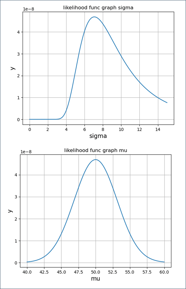

なお、正規分布の公式やグラフは、以下の記事を参照のこと。

正規分布の計算を行いグラフを描いてみた 正規分布は連続型の確率分布(=確率密度関数)の1つで、世の中の多くの分布が正規分布に従うといわれている。 平均$μ$、分散...

また、二項分布の場合の尤度関数については、以下の記事を参照のこと。

二項分布の尤度関数を計算しグラフ化してみた 二項分布に従うある事象が起こる確率$p$が分からない状態で、$5$回中$3$回ある事象が起きた場合に、最も起こりうる確率...

先ほどの尤度関数
$$\begin{eqnarray} L = \displaystyle \prod_{i=1}^{5} \frac{1}{\sqrt{2π}σ}\exp({-\frac{{(x_i-μ)}^2}{2σ^2}}) \end{eqnarray}$$
が最大になるような平均$μ$、標準偏差$σ$が、最も起こりうる平均$μ$と標準偏差$σ$となるが、この計算は煩雑になるため、二項分布の場合と同様、尤度関数$L$に自然対数をとった対数尤度関数を計算する。

$$\begin{multline} logL = log(\displaystyle \prod_{i=1}^{5} \frac{1}{\sqrt{2π}σ}\exp({-\frac{{(x_i-μ)}^2}{2σ^2}})) \\ \shoveleft{　　　= log(\frac{1}{\sqrt{2π}σ}\exp({-\frac{{(x_1-μ)}^2}{2σ^2}})) \times log(\frac{1}{\sqrt{2π}σ}\exp({-\frac{{(x_2-μ)}^2}{2σ^2}})) } \\ \shoveleft{　　　　　\times ･･･ \times log(\frac{1}{\sqrt{2π}σ}\exp({-\frac{{(x_5-μ)}^2}{2σ^2}})) } \\ \shoveleft{　　　= log(\frac{1}{\sqrt{2π}σ}) + log(\exp({-\frac{{(x_1-μ)}^2}{2σ^2}})) + log(\frac{1}{\sqrt{2π}σ}) + log(\exp({-\frac{{(x_2-μ)}^2}{2σ^2}})) } \\ \shoveleft{　　　　　+ ･･･ + log(\frac{1}{\sqrt{2π}σ}) + log(\exp({-\frac{{(x_5-μ)}^2}{2σ^2}})) } \\ \shoveleft{　　　= \displaystyle \sum_{i=1}^{5} \left\{log(\frac{1}{\sqrt{2π}σ}) + log(\exp({-\frac{{(x_i-μ)}^2}{2σ^2}})\right\}} \\ \shoveleft{　　　= \displaystyle \sum_{i=1}^{5} \left\{log(\frac{1}{\sqrt{2π}σ}) – \frac{{(x_i-μ)}^2}{2σ^2} \right\}} \end{multline}$$

この対数尤度関数$logL$を、平均$=50$ または 標準偏差$=7$ で固定化してグラフ化した結果は以下のようになり、尤度関数の時と同様、$x_i=40$, $45$, $50$, $55$, $60$の平均・標準偏差の値付近で最大になることが確認できる。

%matplotlib inline
import numpy as np
import matplotlib.pyplot as plt

# 対数の正規分布の計算
# 引数のaveは平均、stdは標準偏差を表す
def log_normal_distribution(x, ave, std):
    ret = np.log(1 / (np.sqrt(2 * np.pi) * std))
    ret = ret - ((x - ave)** 2) / (2 * (std**2))
    return ret

# 4～15までを1000等分した値をsigmaとする
sigma = np.linspace(4, 15, 1000)
# 平均=50で固定し、標準偏差をsigmaとして、
# x=40,45,50,55,60の場合を全て足した対数尤度関数の値を計算
y1 = log_normal_distribution(40, 50, sigma)
y2 = log_normal_distribution(45, 50, sigma)
y3 = log_normal_distribution(50, 50, sigma)
y4 = log_normal_distribution(55, 50, sigma)
y5 = log_normal_distribution(60, 50, sigma)
y = y1 + y2 + y3 + y4 + y5
plt.plot(sigma, y)
plt.title("log likelihood func graph sigma")
plt.xlabel("sigma", size=14)
plt.ylabel("y", size=14)
plt.grid()
plt.show()

# 40～60までを1000等分した値をmuとする
mu = np.linspace(40, 60, 1000)
# 標準偏差=7で固定し、平均をmuとして、
# x=40,45,50,55,60の場合を全て足した対数尤度関数の値を計算
y1 = log_normal_distribution(40, mu, 7)
y2 = log_normal_distribution(45, mu, 7)
y3 = log_normal_distribution(50, mu, 7)
y4 = log_normal_distribution(55, mu, 7)
y5 = log_normal_distribution(60, mu, 7)
y = y1 + y2 + y3 + y4 + y5
plt.plot(mu, y)
plt.title("log likelihood func graph mu")
plt.xlabel("mu", size=14)
plt.ylabel("y", size=14)
plt.grid()
plt.show()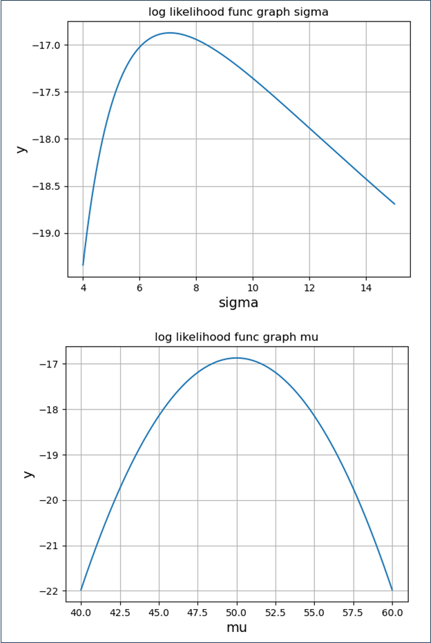

サラリーマン型フリーランスSEという働き方でお金の不安を解消しよう先日、「サラリーマン型フリーランスSE」という働き方を紹介するYouTube動画を視聴しましたので、その内容をご紹介します。 「サ...

さらに、対数尤度関数$logL$が最大になる$μ$,$σ$は、$logL$を$μ$,$σ$それぞれについて偏微分して計算した値がゼロになる値となる。
$$\begin{multline} \displaystyle \frac{\partial}{\partial μ}logL = \frac{\partial}{\partial μ} \displaystyle \sum_{i=1}^{5} \left\{log(\frac{1}{\sqrt{2π}σ}) – \frac{{(x_i-μ)}^2}{2σ^2} \right\} \\ \shoveleft{　　　　　= \displaystyle \sum_{i=1}^{5} \left\{ \frac{\partial}{\partial μ}log(\frac{1}{\sqrt{2π}σ}) – \frac{\partial}{\partial μ}\frac{{(x_i-μ)}^2}{2σ^2} \right\}} \\ \shoveleft{　　　　　= \displaystyle \sum_{i=1}^{5} \left\{ 0 – \frac{1}{2σ^2} \times \frac{\partial}{\partial μ}(x_i-μ)^2 \right\}} \\ \shoveleft{　　　　　= \displaystyle \sum_{i=1}^{5} \left\{ – \frac{1}{2σ^2} \times 2(x_i-μ) \times (-1) \right\}} \\ \shoveleft{　　　　　= \displaystyle \sum_{i=1}^{5} \left\{ \frac{x_i-μ}{σ^2} \right\}} \\ \shoveleft{　　　　　= \frac{\displaystyle \sum_{i=1}^{5}x_i – 5μ}{σ^2}} \end{multline}$$
この値が$0$になる$μ$を計算すると、以下の通り、$5$つの値$40$, $45$, $50$, $55$, $60$の平均値となる。
$$\begin{eqnarray} \frac{\displaystyle \sum_{i=1}^{5}x_i – 5μ}{σ^2} &=& 0 \\ \displaystyle \sum_{i=1}^{5}x_i – 5μ &=& 0 \\ 5μ &=& \displaystyle \sum_{i=1}^{5}x_i \\ 5μ &=& (40 + 45 + 50 + 55 + 60) \\ 5μ &=& 250 \\ μ &=& 50 \end{eqnarray}$$
同様に、
$$\begin{multline} \displaystyle \frac{\partial}{\partial σ}logL = \frac{\partial}{\partial σ} \displaystyle \sum_{i=1}^{5} \left\{log(\frac{1}{\sqrt{2π}σ}) – \frac{{(x_i-μ)}^2}{2σ^2} \right\} \\ \shoveleft{　　　　　= \displaystyle \sum_{i=1}^{5} \left\{ \frac{\partial}{\partial σ}log{\frac{1}{\sqrt{2π}σ}} – \frac{\partial}{\partial σ}\frac{{(x_i-μ)}^2}{2σ^2} \right\}} \\ \shoveleft{　　　　　= \displaystyle \sum_{i=1}^{5} \left\{ \frac{\partial}{\partial σ}log({2πσ^2})^{-\frac{1}{2}} – {(x_i-μ)}^2 \times \frac{\partial}{\partial σ}\frac{1}{2σ^2} \right\}} \\ \shoveleft{　　　　　= \displaystyle \sum_{i=1}^{5} \left\{ -\frac{1}{2} \times \frac{\partial}{\partial σ}log({2πσ^2}) – {(x_i-μ)}^2 \times \frac{\partial}{\partial σ}(2σ^2)^{-1} \right\}} \\ \shoveleft{　　　　　= \displaystyle \sum_{i=1}^{5} \left\{ -\frac{1}{2} \times \frac{1}{2πσ^2} \times 4πσ + {(x_i-μ)}^2 \times (2σ^2)^{-2} \times 4σ \right\}} \\ \shoveleft{　　　　　= \displaystyle \sum_{i=1}^{5} \left\{ -\frac{4πσ}{4πσ^2} + \frac{{(x_i-μ)}^2 \times 4σ}{4σ^4} \right\}} \\ \shoveleft{　　　　　= \displaystyle \sum_{i=1}^{5} \left\{ -\frac{1}{σ} + \frac{{(x_i-μ)}^2}{σ^3} \right\}} \end{multline}$$
この値が$0$になる$σ$を計算すると、以下の通り、$5$つの値$40$, $45$, $50$, $55$, $60$の標準偏差となる。
$$\begin{eqnarray} \displaystyle \sum_{i=1}^{5} \left\{ -\frac{1}{σ} + \frac{{(x_i-μ)}^2}{σ^3} \right\} &=& 0 \\ -\frac{5}{σ} + \frac{\sum_{i=1}^{5}{(x_i-μ)}^2}{σ^3} &=& 0 \\ -5σ^2 + \sum_{i=1}^{5}{(x_i-μ)}^2 &=& 0 \\ -5σ^2 &=& -\sum_{i=1}^{5}{(x_i-μ)}^2 \\ σ^2 &=& \frac{\sum_{i=1}^{5}{(x_i-μ)}^2}{5} \\ σ^2 &=& \frac{{(40-50)}^2 + {(45-50)}^2 + {(50-50)}^2 + {(55-50)}^2 + {(60-50)}^2}{5} \\ σ^2 &=& \frac{100 + 25 + 0 + 25 + 100}{5} \\ σ^2 &=& \frac{250}{5} \\ σ^2 &=& 50 \\ σ &=& \sqrt{50} = 5\sqrt{2} ≒ 7.07 \end{eqnarray}$$

要点まとめ

• 想定するパラメーターがある値をとる場合に、観測している事柄や事象が起こりうる確率を表現したものを尤度関数という。
• 尤度関数を計算する際、乗算を多く含むと計算しにくいため、尤度関数$L$に自然対数をとった対数尤度関数を利用する場合も多い。
• 正規分布に従う対数尤度関数の最大値をとる平均$μ$、標準偏差$σ$は、その偏微分が$0$になる値を計算することで求められる。
• 正規分布に従う尤度関数の最大値をとる平均$μ$、標準偏差$σ$は、実際に観測されたデータの平均、標準偏差を計算することで求められる。